Opening a 63 GB Climate Mesh: 300 Million Cells, 306 Seconds
There is a 63 GB file on a DOE cluster describing the finest mesh in a next-generation climate simulation — 200-metre resolution over the continental United States, three hundred million cells. Until last week, the Python stack the climate community actually uses to read these meshes could not open it. Not slowly. At all. Every attempt ended the same way: Remote execution failed, several minutes in, the real error swallowed by the client.
The natural assumption is that a 63 GB file needs more than 63 GB of memory, and you need a bigger machine. That assumption is wrong, and the reason it is wrong is the best thing I learned all month: 86% of that file is the same coordinates, written over and over. The mesh reader was faithfully holding every copy in memory at once to find the 14% that were distinct.
It now opens in 306 seconds. Nothing about the hardware changed.
What a SCRIP file actually stores
The mesh is in SCRIP format — a convention from the Spherical Coordinate Remapping and Interpolation Package, now the lingua franca for telling one climate model what another model’s grid looks like. Its layout is disarmingly simple. For a mesh of grid_size cells, each with up to grid_corners corners, it stores two arrays:
double grid_corner_lon(grid_size, grid_corners)
double grid_corner_lat(grid_size, grid_corners)
That is: for every cell, the longitude and latitude of each of its corners, written out in full.
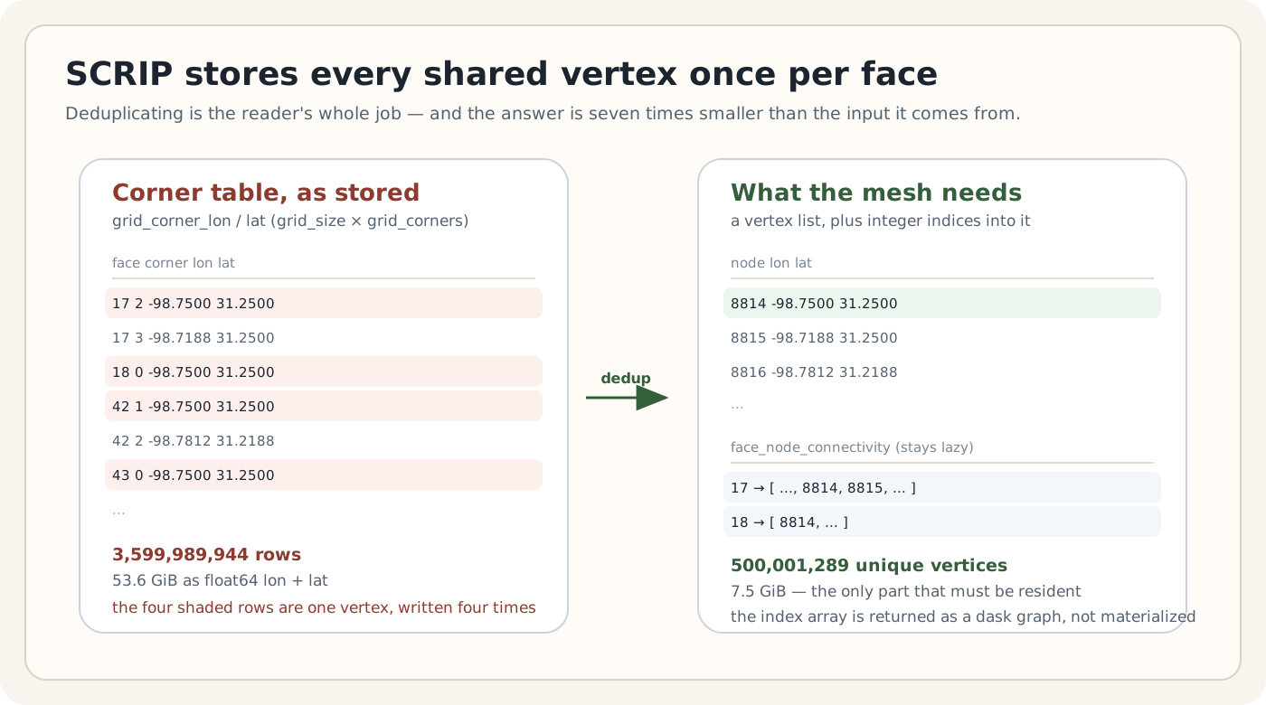
Notice what that means. In any real mesh, cells share vertices — that is what makes it a mesh rather than a pile of disconnected polygons. A quadrilateral grid has roughly four cells meeting at each vertex, so each vertex’s coordinates appear about four times in the file. SCRIP does not store a vertex list and an index into it. It stores the coordinates again, in full, once per face that touches them.
For the file in question:
grid_size (cells) | 299,999,162 |
grid_corners | 12 |
| corner table rows | 3,599,989,944 |
| as float64 lon + lat | 53.6 GiB |
3.6 billion coordinate pairs. And the unique vertices among them turn out to number 500,001,289 — so about 86% of that 53.6 GiB is restatement of coordinates already present elsewhere in the file.
To turn this into a usable mesh — a vertex list plus a connectivity array saying which vertices form which face — a reader has to find those unique vertices and map every corner to its index. That is a deduplication over 3.6 billion rows.
The reader’s approach, and why it hit a wall
UXarray’s SCRIP reader did this with Polars, and the code was perfectly reasonable:
df = pl.DataFrame({"lon": corner_lon, "lat": corner_lat}).with_row_count("original_index")
unique_df = df.unique(subset=["lon", "lat"], keep="first")
...
df_joined = df.join(unique_df.drop("original_index"), on=["lon", "lat"], how="left")
unq_inv = df_joined["unique_id"].to_numpy().astype(INT_DTYPE)
Build a dataframe of every corner, take unique rows, join back to recover which unique vertex each original corner maps to. Polars is fast and this is idiomatic.
The problem is the first line. pl.DataFrame({...}) requires both full arrays in memory, and the join then needs the frame plus its result. For a small mesh this is invisible. For 3.6 billion rows, the frame alone is the 53.6 GiB above, and the join is a multiple of that.
And there was no way to ask for anything else. xarray and UXarray let you open a file lazily by passing chunks=, which hands you dask-backed arrays that read from disk on demand. But the SCRIP reader never dispatched on that — it called np.asarray() on the corner variables, which forces a lazily-opened dask array straight into memory. You could pass chunks="auto" and watch it allocate anyway.
Reproducing it without the cluster
Before writing anything I wanted the failure on a machine I could instrument. The 63 GB file lives only on the cluster, but there was a 24 GB SCRIP file on my laptop — ne2048np4, 226 million cells with 5 corners each, a 1.1-billion-row corner table at 16.9 GiB.
The laptop has 64 GB of RAM. The eager path:
exhausted all 35 GB of swap, killed at ~9 minutes, no result
Which is the same failure as the cluster, three times smaller, on hardware I could watch. Good enough.
The fix: dedup is a shuffle, not a table scan
The key observation is that finding unique rows does not require holding all rows at once. It requires that rows with equal keys meet each other. That is what a shuffle does: partition the data by a hash of the key, so all rows with the same (lon, lat) land in the same partition, then deduplicate each partition independently. Partitions are processed one at a time and can spill to disk.
dask.dataframe implements exactly this, so when the corner arrays arrive dask-backed, the reader can hand the problem over:
coords = dask_array.stack([corner_lon, corner_lat], axis=1)
ddf = dd.from_dask_array(coords, columns=["lon", "lat"])

unique_pairs = (
    ddf.drop_duplicates(subset=["lon", "lat"], keep="first")
    .compute()
    .reset_index(drop=True)
)
The result is the unique table — 500 million rows, 7.5 GiB — which is large but not 53.6 GiB, and is the one thing that genuinely has to be resident.
Then there is the second half, which is easy to get wrong. Every one of the 3.6 billion corners still needs an index into that vertex list. Materializing that as a NumPy array would cost another 26.8 GiB and undo the work. Instead, broadcast the small lookup table across the corner array’s own blocks and leave the result lazy:
unq_inv = dask_array.map_blocks(
    _lookup_node_ids, corner_lon, corner_lat, lookup=lookup, dtype=INT_DTYPE
)
map_blocks, not dask.dataframe.map_partitions — the latter produces output with unknown chunk sizes, while map_blocks preserves the input’s known chunk structure, which everything downstream depends on. The connectivity array stays a dask graph until something actually needs its values.
The eager path is untouched. A small mesh still goes through Polars, because for a small mesh that is faster and the shuffle machinery is pure overhead.
Three things the profiler found that reasoning missed
The fix worked at this point. Then measurement made it 32% cheaper, caught an “optimization” that was making things worse, and found a latent bug that would have silently corrupted every mesh it touched.
A one-line config change worth 32% of peak memory
dask picks a shuffle implementation based on what’s available. Without a distributed client in the process, the default it chose was a wholly in-memory shuffle — which is precisely the thing being avoided. Pinning it to the disk method:
| shuffle | peak RSS on the 226M-cell mesh |
|---|---|
| dask’s default | 17.9 GiB |
disk, explicitly | 12.1 GiB |
Identical output, a third less memory, one line. Only when nobody has chosen otherwise, though — with a real distributed cluster, dask’s peer-to-peer shuffle is the better choice and overriding it would be wrong:
if dask.config.get("dataframe.shuffle.method", None) is None:
    if not _distributed_client_active():
        shuffle_cfg["dataframe.shuffle.method"] = "disk"
The optimization that made it worse
Profiling the stages showed peak memory well above what the shuffle alone explained. Three copies of the unique-vertex table were alive simultaneously: the pandas frame from .compute(), the two NumPy arrays extracted from it, and the Polars lookup built from those. At 3.4 GiB each on the local mesh, that is not a rounding error.
My first attempt was to_numpy(copy=True), reasoning that an explicit copy would let the parent frame be freed. Measured: peak went up, 23.9 → 26.5 GiB. The copy was real; the frame was not freed any sooner. Dropping it with del instead took 31.0 → 29.3 GiB, across three runs each way.
The argument for copy=True was clean and it was wrong. At this scale that is the norm, not the exception — which is why every number in this post is measured rather than derived.
The bug that would never have crashed
The per-block function joins corner coordinates against the lookup table to get vertex ids. map_blocks requires the output block to stay positionally aligned with its input — element i out must correspond to element i in.
Polars’ documentation says, of join ordering: “Do not rely on any observed ordering without explicitly setting this parameter, as your code may break in a future release.”
So I sabotaged it: removed the ordering guarantee and ran the entire test suite. Everything passed.
Which means the guarantee was load-bearing and untested, and a future Polars release could reorder that join without a single red test anywhere. The failure mode is not a crash — it is every cell in a 300-million-cell mesh built from the wrong vertices. Areas wrong. Surface normals flipped. Results that look completely plausible and are completely false.
So the requirement is now stated rather than assumed:
joined = block.join(lookup, on=["lon", "lat"], how="left", maintain_order="left")
And the tests were rewritten until they could actually catch it — confirmed by breaking the code on purpose and watching six of them fail. The old tests compared corner coordinates sorted per face, which is blind to a winding-order change, and winding determines the sign of a cell’s area. They now compare in winding order.
If you take one habit from this post, take that one: break your fix deliberately and confirm the suite goes red. A test that cannot fail is documentation wearing a lab coat.
Results
Start with a 24 GB mesh — 226 million cells — on a 64 GB laptop. The old path never finishes:
| path | outcome |
|---|---|
| eager | exhausts 35 GB of swap, killed after 9 minutes |
| lazy | 60 seconds, 29 GiB peak |
Then the real target. 63 GB, on a cluster node:
| cells | 299,999,162 |
| unique vertices | 500,001,289 |
| wall time | 306 s |
| peak memory | 117.7 GiB |
Three hundred million cells and half a billion vertices, resolved in five minutes, on a file that had defeated every attempt before this. The deduplication itself took 135 s at 38.1 GiB; the rest is assembling connectivity and coordinates for 3.6 billion corners.
Worth knowing before you try it: 117.7 GiB is a compute-node number, not a laptop one. The point is not that the file became small — it is that it became possible, and the memory it needs is now proportional to the mesh’s actual information content rather than to how many times the format repeated itself.
And reading is not the same as working with. A bounding-box subset of this same file still will not run, for a reason that has nothing to do with the corner table: cropping needs a per-face bounding box for every face before it can test which ones fall inside the box, and on the twin mesh that index measured 109 GiB on its own. Scaled up it wants roughly 363 GiB against a 236 GiB node, and asking for a smaller box does not help — the index is built before the box is consulted. Two orders of magnitude of duplicate coordinates were the thing standing between this file and being readable. Something else stands between readable and useful, and it is a different problem.
And one number makes the whole approach predictable. Peak memory landed at 0.71× the corner table at both scales — 12.1 GiB against 16.9 GiB on the laptop, 38.1 GiB against 53.6 GiB on the cluster. A ratio that holds across a 3× change in size is what let the laptop measurement predict the cluster run before anyone spent a node-hour on it. If you are sizing a job like this, that constant is the useful export from this whole exercise.
Why 12 corners, and a physical aside
The 12 in grid_corners is not arbitrary, and it explains why this particular file is the one that broke.
Spectral-element atmosphere models carry their state at Gauss–Lobatto–Legendre quadrature points inside each element. An np4 configuration has a 4×4 grid of these per element. Writing that to SCRIP — a format that only knows how to describe polygonal cells — produces a dual-cell decomposition where cells can have up to 12 corners.
Its pg2 sibling describes the same physical mesh as 4-cornered finite-volume cells: 133 million cells, 12 GB, and it always opened fine. A physical field lives on pg2. There is no reason to load the np4 file to make a picture.
The dedup ratios make the structural difference visible:
| mesh | corners/face | unique nodes / corner rows | nodes per face |
|---|---|---|---|
ne2048np4 (5 corners) | 5 | 0.200 | 1.00 |
1024x4-np4 (12 corners) | 12 | 0.139 | 1.67 |
Exactly 1.00 nodes per face in the first is the signature of a quadrilateral cubed-sphere grid where the vertex and cell counts coincide. The second’s 1.67 reflects the GLL decomposition’s more complicated sharing pattern. Neither number is something you’d guess; both fall out of the dedup and are a decent sanity check that the reader did the right thing.
If you have one of these files
The practical version, for someone who has a large SCRIP mesh and a job to do rather than a reader to write.
Check which encoding you actually need first. The mesh in this post ships in two forms describing the same geometry: np4 (12 corners per face, 63 GB) and pg2 (4 corners, 12 GB). A physics field lives on pg2. Everything below is cheaper on it by roughly a factor of four, and nothing about the science is lost. The directory’s own README said so, and the expensive way to learn it is to spend a day on the other file.
Expect these costs, measured on a 236 GiB compute node:
| operation | 133M faces (pg2) | 300M faces (np4) |
|---|---|---|
| open + read topology | 33 GiB | 119 GiB |
| + per-face bounding boxes | 142 GiB | ~363 GiB — does not fit |
| bounding-box subset | works, 113 s | no |
Reading a mesh and working with one are different problems. The dedup fix in this post made the 63 GB file readable. Cropping it to a region still does not run, because a bounding-box subset first computes a bounding box for every face in the mesh — all 300 million — before it can test which ones fall inside your box. Asking for a smaller region does not help: the index is built before the box is consulted. I tried a half-degree box around Austin and it died at exactly the same point as a box covering all of Texas.
Pick the remap method for your field, not from a table. All seven methods available here were measured on the same grid pair, and the ranking inverts depending on what you are remapping:
| smooth field | field with a front | |
|---|---|---|
| conservative (YAC) | 0.095% | 0.416% |
| dnn (YAC) | 0.062% | 0.452% |
| inverse distance weighted | 0.075% | 1.49% |
| bilinear | 0.083% | 2.48% |
| nearest neighbour | 0.204% | 7.14% |
On something smooth, nearly anything works and the smoothers edge ahead. On a discontinuity — a front, a coastline, an orographic band, precipitation — conservative wins by 3.6x over the next non-YAC method and 17x over nearest neighbour. Real fields have fronts. A benchmark on a smooth analytic field will rank these methods in an order that does not survive contact with your data, which is worth knowing before you trust one.
The pattern, past SCRIP files
Five things worth stealing:
- If an operation only needs equal keys to meet, it’s a shuffle, not a scan. Deduplication, group-by, join — all are partitionable by hash of the key, and all can run in bounded memory over unbounded input. If your library only offers the in-memory version, the out-of-core one usually exists a layer down.
- Keep the large derived thing lazy. The unique vertices had to be materialized. The 3.6-billion-element index into them did not, and returning it as a dask array rather than a NumPy array is most of the difference between fitting and not.
- Don’t replace the fast path. Small meshes still go through Polars. An out-of-core algorithm that is universally slower is a regression wearing a fix’s clothes.
- Measure the optimization you just reasoned your way to. One of my three memory changes made things worse and I would have shipped it on the strength of the argument alone.
- Ask whether your test can fail. Removing the ordering guarantee broke nothing, which meant the test was decorative. Sabotage is a cheap way to find out.
Three hundred and fifty lines, tests included. That is what stood between three hundred million cells and every tool that wanted to read them.
The standing advice had been to use the coarser file instead, and it was sensible advice — but “use the coarser file” and “our tools cannot open this file” are very different sentences, and only the first one is about the science. The resolution was always in the data. Nothing needed to be bought, provisioned, or waited for. It needed someone to notice that most of a 53.6 GiB array was the same numbers, over and over, and that nothing required them all to be in memory at the same time.
The changes are in UXarray#1775, against issue #1774.